b = fir2( n , f,m ) returns an n th-order FIR filter with frequency-magnitude characteristics specified in the vectors f and m . The function linearly interpolates the desired frequency response onto a dense grid and then uses the inverse Fourier transform and a Hamming window to obtain the filter coefficients.
b = fir2( n , f,m , npt , lap ) specifies npt , the number of points in the interpolation grid, and lap , the length of the region that fir2 inserts around duplicate frequency points which specify steps in the frequency response.
b = fir2( ___ , window ) specifies a window vector to use in the design in addition to any input arguments from previous syntaxes.
Note: Use fir1 for window-based standard lowpass, bandpass, highpass, bandstop, and multiband configurations.
Load the MAT-file chirp . The file contains a signal, y , sampled at a frequency Fs = 8192 Hz. The signal has most of its power above Fs /4 = 2048 Hz, or half the Nyquist frequency. Add random noise to the signal.
load chirp y = y + randn(size(y))/25; t = (0:length(y)-1)/Fs;
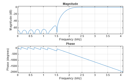
Design a 34th-order FIR highpass filter to attenuate the components of the signal below Fs /4. Specify a normalized cutoff frequency of 0.48, which corresponds to about 1966 Hz. Visualize the frequency response of the filter.
f = [0 0.48 0.48 1]; mhi = [0 0 1 1]; bhi = fir2(34,f,mhi); freqz(bhi,1,[],Fs)
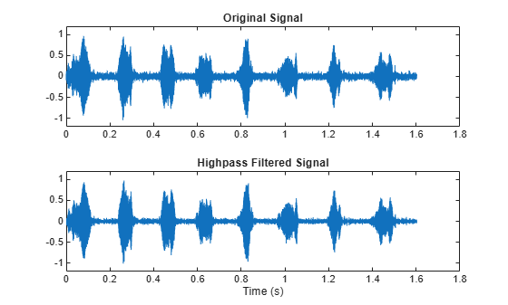
Filter the chirp signal. Plot the signal before and after filtering.
outhi = filter(bhi,1,y); figure subplot(2,1,1) plot(t,y) title('Original Signal') ylim([-1.2 1.2]) subplot(2,1,2) plot(t,outhi) title('Highpass Filtered Signal') xlabel('Time (s)') ylim([-1.2 1.2])
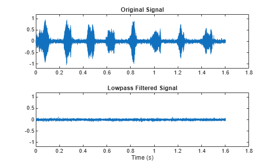
Change the filter from highpass to lowpass. Use the same order and cutoff. Filter the signal again. The result is mostly noise.
mlo = [1 1 0 0]; blo = fir2(34,f,mlo); outlo = filter(blo,1,y); subplot(2,1,1) plot(t,y) title('Original Signal') ylim([-1.2 1.2]) subplot(2,1,2) plot(t,outlo) title('Lowpass Filtered Signal') xlabel('Time (s)') ylim([-1.2 1.2])
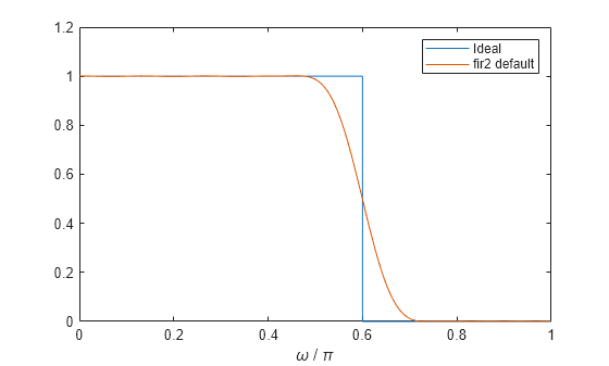
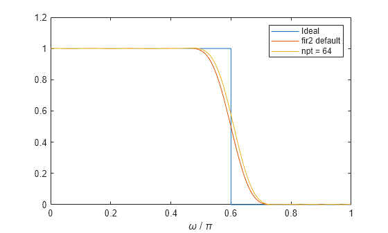
Design a 30th-order lowpass filter with a normalized cutoff frequency of 0 . 6 π rad/sample. Plot the ideal frequency response overlaid with the actual frequency response.
f = [0 0.6 0.6 1]; m = [1 1 0 0]; b1 = fir2(30,f,m); [h1,w] = freqz(b1,1); plot(f,m,w/pi,abs(h1)) xlabel('\omega / \pi') lgs = 'Ideal','fir2 default'>; legend(lgs)
Redesign the filter using a 64-point interpolation grid.
b2 = fir2(30,f,m,64); h2 = freqz(b2,1); hold on plot(w/pi,abs(h2)) lgs = 'npt = 64'; legend(lgs)
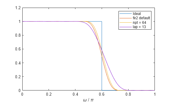
Redesign the filter using the 64-point interpolation grid and a 13-point interval around the cutoff frequency.
b3 = fir2(30,f,m,64,13); h3 = freqz(b3,1); plot(w/pi,abs(h3)) lgs = 'lap = 13'; legend(lgs)
Design an FIR filter with the following frequency response:
F1 = 0:0.01:0.18; A1 = 0.5+sin(2*pi*7.5*F1)/4;
F2 = [0.2 0.38 0.4 0.55 0.562 0.585 0.6 0.78]; A2 = [0.5 2.3 1 1 -0.2 -0.2 1 1];
F3 = 0.79:0.01:1; A3 = 0.2+18*(1-F3).^2;
Design the filter using a Hamming window. Specify a filter order of 50.
N = 50; FreqVect = [F1 F2 F3]; AmplVect = [A1 A2 A3]; ham = fir2(N,FreqVect,AmplVect);
Repeat the calculation using a Kaiser window that has a shape parameter of 3.
kai = fir2(N,FreqVect,AmplVect,kaiser(N+1,3));
Redesign the filter using the designfilt function. designfilt uses a rectangular window by default. Compute the zero-phase response of the filter over 1024 points.
d = designfilt('arbmagfir','FilterOrder',N, . 'Frequencies',FreqVect,'Amplitudes',AmplVect); [zd,wd] = zerophase(d,1024);
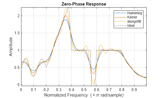
Display the zero-phase responses of the three filters. Overlay the ideal response.
zerophase(ham,1) hold on zerophase(kai,1) plot(wd/pi,zd) plot(FreqVect,AmplVect,'k:') legend('Hamming','Kaiser','designfilt','ideal')
Filter order, specified as an integer scalar.
For configurations with a passband at the Nyquist frequency, fir2 always uses an even order. If you specify an odd-valued n for one of those configurations, then fir2 increments n by 1.
Data Types: double
Frequency-magnitude characteristics, specified as vectors of the same length.
Data Types: double
Number of grid points, specified as a positive integer scalar. npt must be larger than one-half the filter order: npt > n /2.
Data Types: double
Length of region around duplicate frequency points, specified as a positive integer scalar.
Data Types: double
Window, specified as a column vector. The window vector must have n + 1 elements. If you do not specify window , then fir2 uses a Hamming window. For a list of available windows, see Windows.
fir2 does not automatically increase the length of window if you attempt to design a filter of odd order with a passband at the Nyquist frequency.
Example: kaiser(n+1,0.5) specifies a Kaiser window with shape parameter 0.5 to use with a filter of order n .
Example: hamming(n+1) is equivalent to leaving the window unspecified.
Data Types: double
Filter coefficients, returned as a row vector of length n + 1. The coefficients are sorted in descending powers of the Z-transform variable z:
fir2 uses frequency sampling to design filters. The function interpolates the desired frequency response linearly onto a dense, evenly spaced grid of length npt . fir2 also sets up regions of lap points around repeated values of f to provide steep but smooth transitions. To obtain the filter coefficients, the function applies an inverse fast Fourier transform to the grid and multiplies by window .
[1] Jackson, L. B. Digital Filters and Signal Processing. 3rd Ed. Boston: Kluwer Academic Publishers, 1996.
[2] Mitra, Sanjit K. Digital Signal Processing: A Computer Based Approach. New York: McGraw-Hill, 1998.
Usage notes and limitations:
All inputs must be constants. Expressions or variables are allowed if their values do not change.
Introduced before R2006a